Measuring Property Gradients

Abstract

Deep learning models achieve high predictive performance but lack intrinsic interpretability, hindering our understanding of the learned prediction behavior. Existing local explainability methods focus on associations, neglecting the causal drivers of model predictions. Other approaches adopt a causal perspective but primarily provide global, model-level explanations. However, for specific inputs, it's unclear whether globally identified factors apply locally. 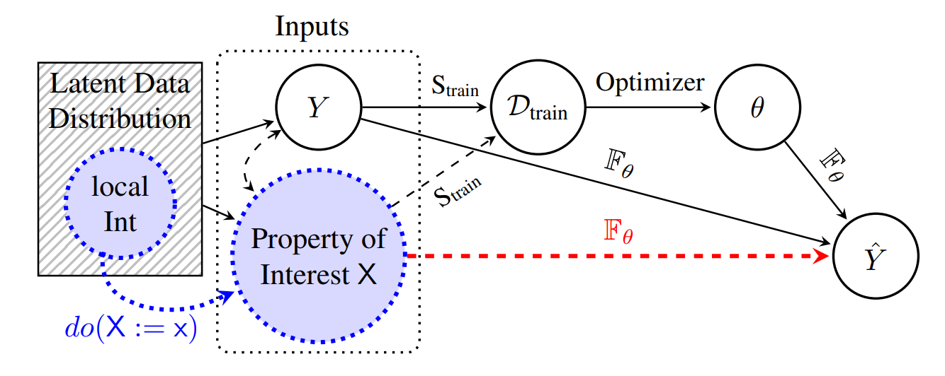To address this limitation, we introduce a novel framework for local interventional explanations by leveraging recent advances in image-to-image editing models. 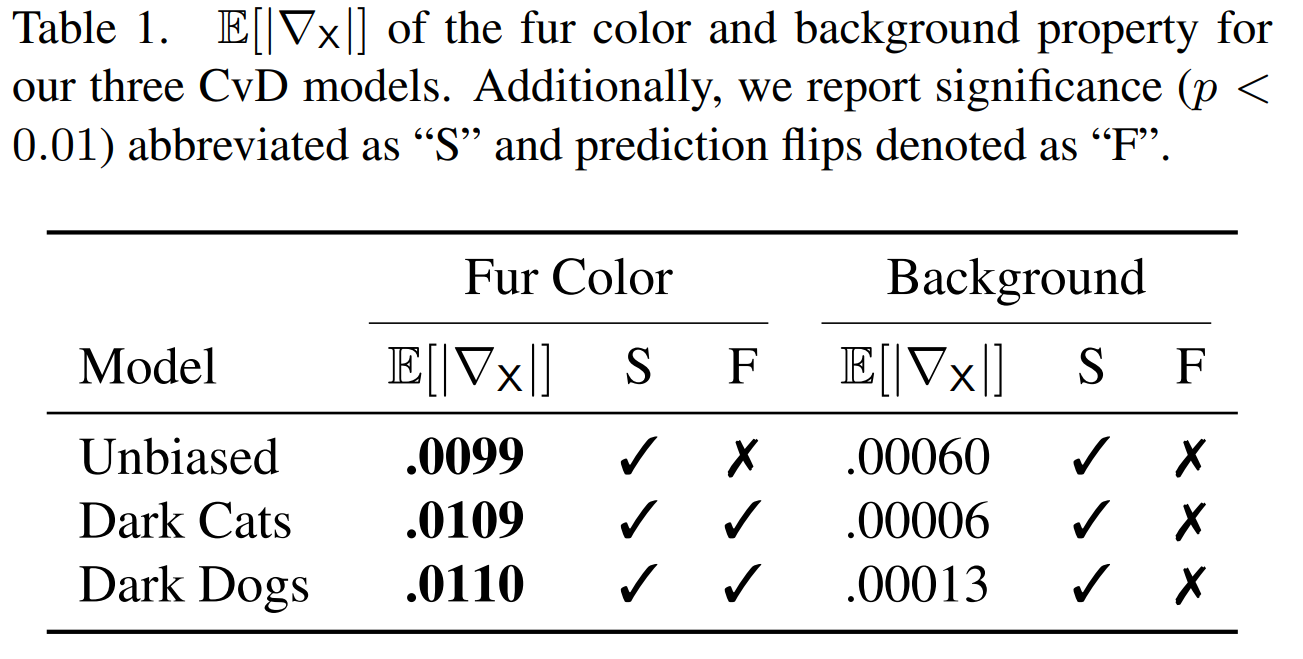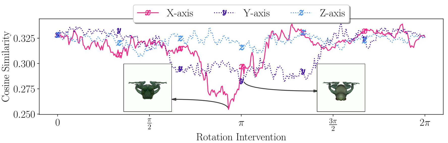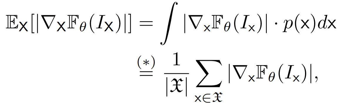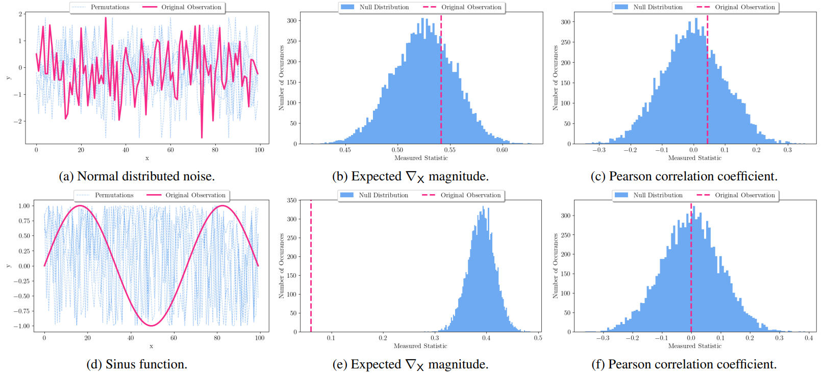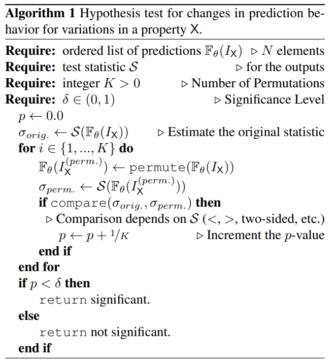Our approach performs gradual interventions on semantic properties to quantify the corresponding impact on a model's predictions using a novel score, the expected property gradient magnitude. We demonstrate the effectiveness of our approach through an extensive empirical evaluation on a wide range of architectures and tasks. 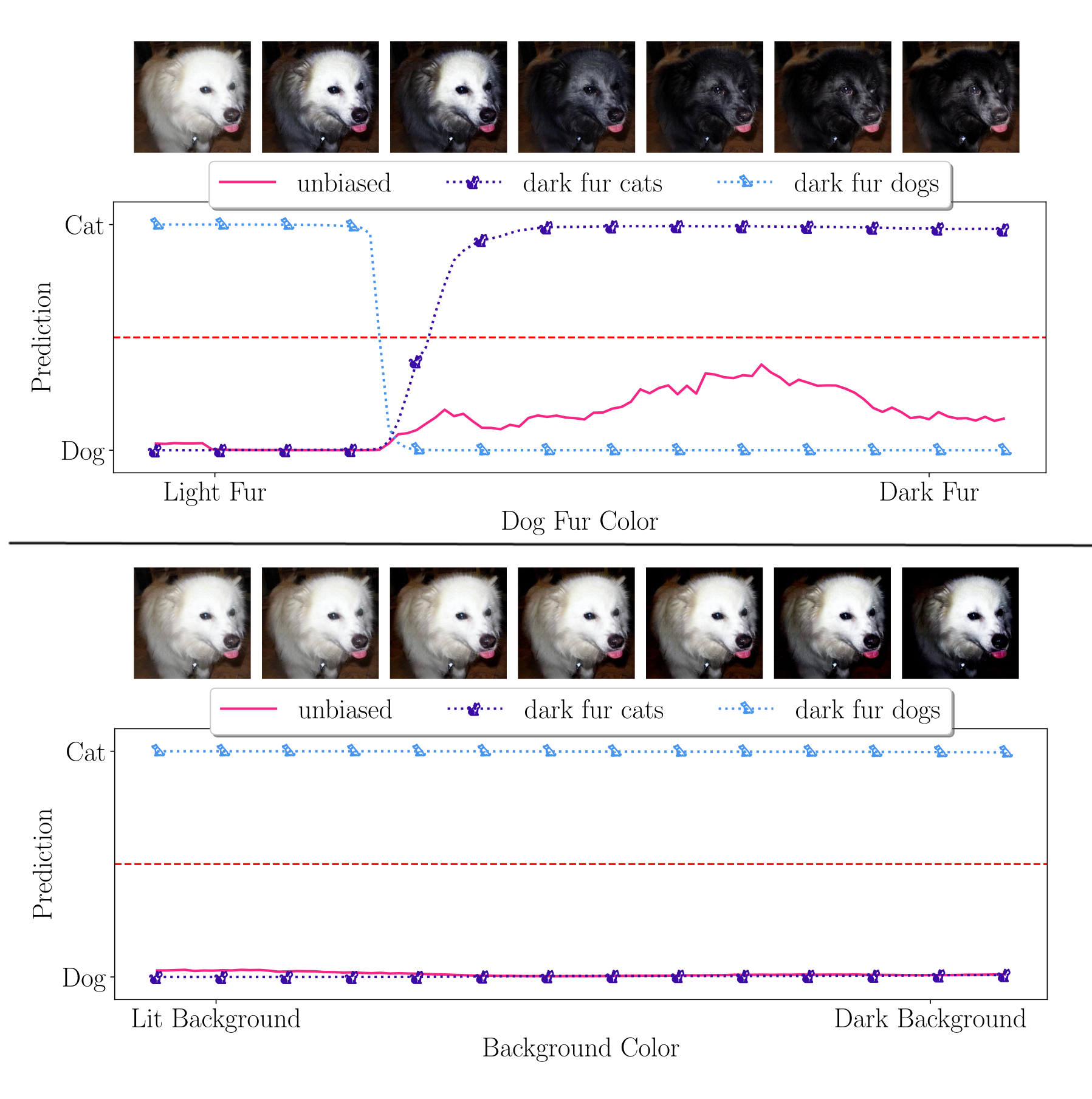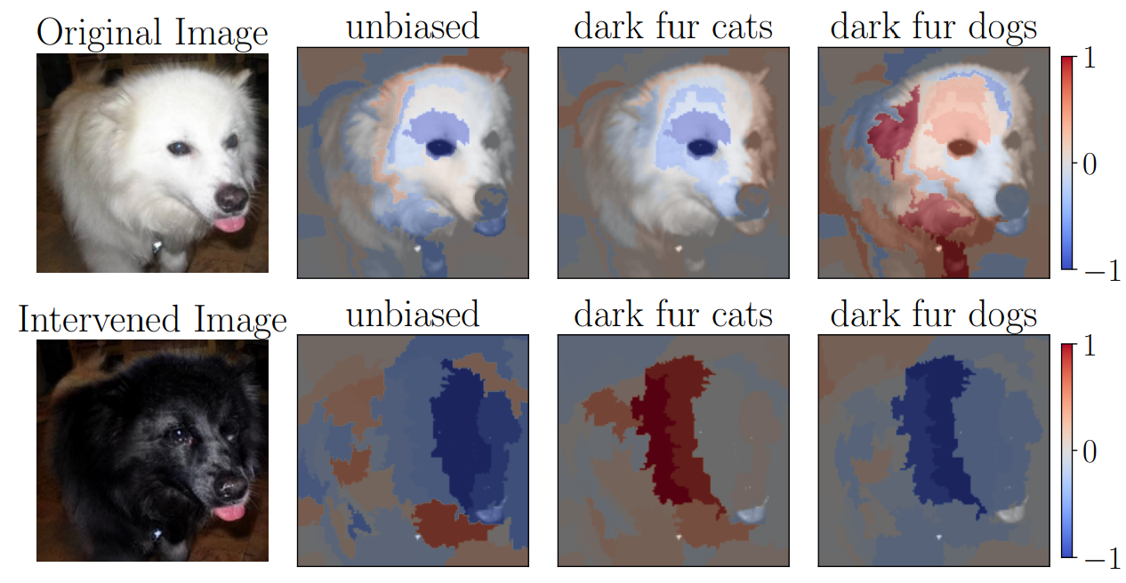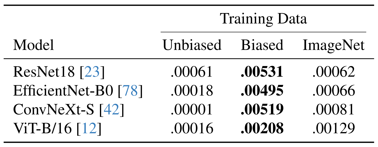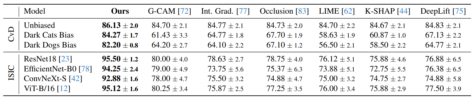First, we validate it in a synthetic scenario and demonstrate its ability to locally identify biases. 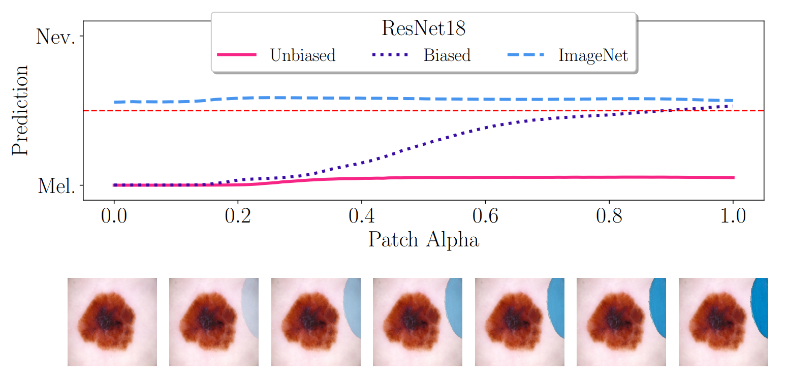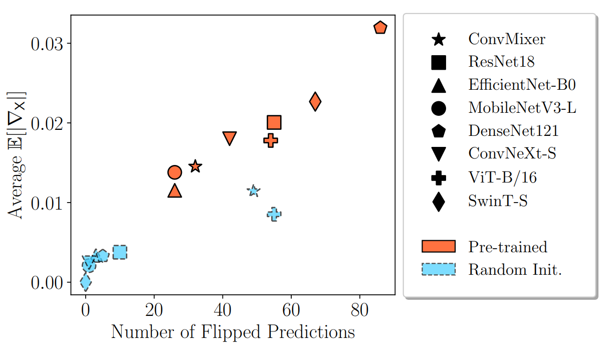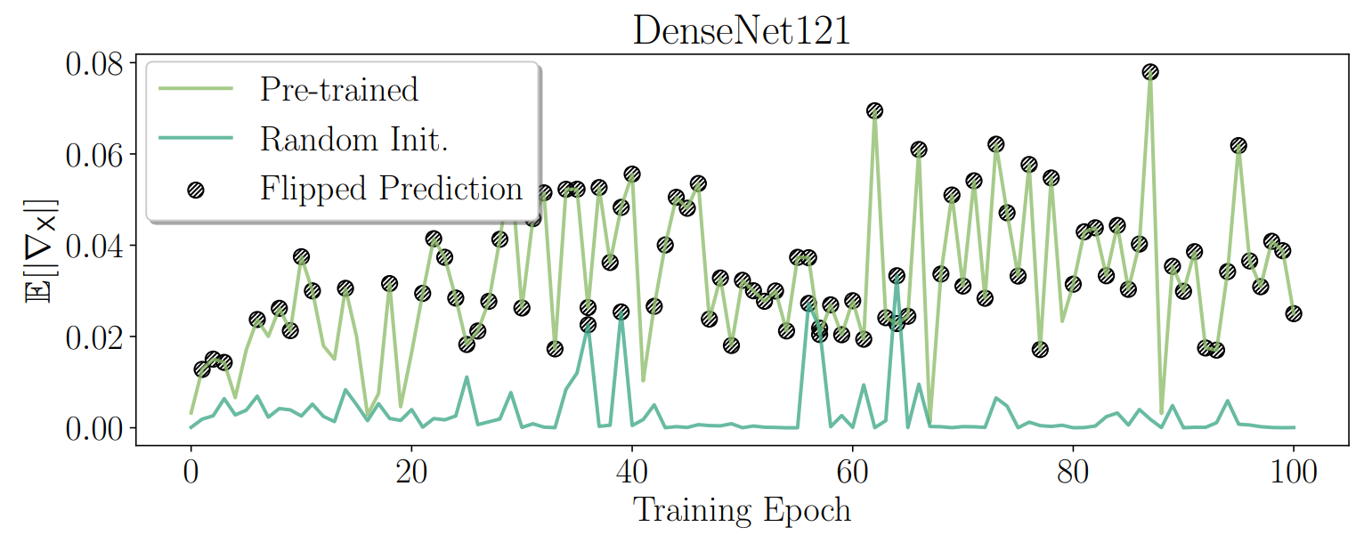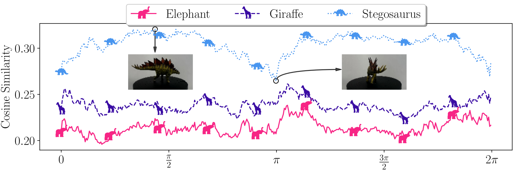Afterward, we apply our approach to investigate medical skin lesion classifiers, analyze network training dynamics, and study a pre-trained CLIP model with real-life interventional data. Our results highlight the potential of interventional explanations on the property level to reveal new insights into the behavior of deep models.

Example Interventions for
Three Cat vs. Dog Classifiers

Important: We first include some results and highlights. You can find a overview for the theoretical foundation further down or simply open our paper 😇

Selected Results and Visualizations

Validation in a Cats versus Dogs Classification Task With Known Bias

We validate our approach in a synthetic scenario with known biases. Specifically, we train models on modified version of the Cats vs. Dogs dataset, where we introduce a spurious correlation between the class label and the animals fur color. In particular, we obtain three training and test data splits: the original unbiased split, a split with only dark-furred dogs and light-furred cats, and the reverse. Our results demonstrate that our method can effectively identify the biased property (fur color) as significant for all three models, while correctly recognizing other properties (e.g., background brightness) as unimportant (see teaser figure above). Further, we can quantify the impact of the property on model predictions (below left), confirming the ability of our approach to detect locally present biases in model predictions.

Our Approach to Quantify Impact

LIME as a Local Attribution Baseline

Crucially, while other local attribution methods highlight important areas, they require semantic interpretation. For example, although the LIME explanations above align with fur color for biased models, the distinction from the unbiased model is unclear. A focus on interventions, i.e., the disparity between the top and bottom rows above left, can help interpret the results. You can find more comparisons and additional baselines in our paper.

Manual Interventions to Study Skin Lesion Classifiers

In the domain of skin lesion classification, a known bias is the correlation between colorful patches and the healthy nevus class. We assess how strongly this property is learned by four different ImageNet pretrained architectures. Then, we either fine-tune on biased skin lesion data (50% nevi with colorful patches) or unbiased data (no patches) from the ISIC archive. To demonstrate that our approach accommodates diverse sources of interventional data, we build on domain knowledge and intervene synthetically. Specifically, we blend segmented colorful patches into melanoma images.

Visualized Average Behavior for ResNet18

Estimated Impact for Different Melanoma Classifiers Trained on Different Data Sources

The mean expected property gradient magnitudes in the table above show that models trained on biased data are most impacted by colorful patch interventions, indicating they learn the statistical correlation between the patches and the nevus class. Furthermore, the variants with ImageNet weights show higher patch sensitivity than the unbiased skin lesion models. We hypothesize this is because learning color is beneficial for general-purpose pre-training, whereas the unbiased models learn to disregard patches and focus on the actual lesions.

Quantitative Comparisons

To quantitatively compare our approach to local baselines, we propose a downstream task inspired by insertion/deletion tests: predicting whether an intervention on a property will change the model's output. This task directly assesses if a method can indicate locally biased behavior and allows for a quantitative comparison to local baselines, given that our approach does not produce saliency maps but rather estimates the impact of a property directly using property gradients. To adapt saliency methods, we measure the mean squared difference of the explanation pre- and post-intervention. For a fair comparison, we select the optimal threshold maximizing the accuracy for both the local baselines and our score.

Our results show that our approach outperforms all local baselines in both the synthetically biased cats versus dogs dataset and the realistic skin lesion task. However, our aim is not to replace saliency methods, but rather to offer a complementary, interventional viewpoint for analyzing local behavior. We demonstrate these capabilities with our analysis of neural network training and CLIP models.

Analyzing Neural Network Training Dynamics

In this section, we analyze the training dynamics of neural networks using our proposed interventional framework. Specifically, we investigate how the sensitivity of a model to a selected property evolves during training. We select a range of convolutional and transformer-based architectures widely used in computer vision tasks. For all of these models, we train a randomly initialized and an ImageNet pre-trained version for 100 epochs.

Regarding the corresponding task, we construct a binary classification problem from CelebA, following an idea proposed in here. Specifically, we utilize the attribute young as a label and split the data in a balanced manner. For this label, the gray hair property is negatively correlated, and a well-performing classifier should learn this association during the training process. To study the training dynamics, we intervene on the hair color and calculate expected property gradient magnitudes after each epoch.

We visualize the average expected property gradient magnitudes of the hair color for a local example over the training process for both pre-trained and randomly initialized models. Specifically, we display the average against the observed flips in the prediction during the hair color intervention (above left). Our analysis reveals two key insights:

First, for all architectures, the pre-trained variants locally exhibit higher expected property gradient magnitudes compared to the randomly initialized versions. This observation is consistent with the number of times the networks' predictions flip during training. In general, we find that increased measured impact correlates with more flipped predictions (above left).
Our second key finding is illustrated in the visualization above right, which reveals that the impact of the hair color exhibits strong local fluctuations during the training for the DenseNets. In other words, the networks do not continuously learn to rely on the hair color property but instead locally "forget" it, even in later epochs. This effect is particularly pronounced for the pre-trained model, whereas the randomly initialized version tends to show lower expected property gradient magnitudes. We observe similar behavior for other architectures.

Analyzing a CLIP Model with Real World Interventions

In our final set of experiments, we investigate the widely used multimodal backbone CLIP ViT-B/32 for zero-shot classification. Our approach is model-agnostic, requiring only access to model outputs, here cosine similarities in the learned latent space. As the property of interest, we select object orientation, which is a known bias, for example, in ImageNet models. Additionally, we demonstrate a third type of interventional data and capture real-life interventional images. Specifically, we record a rotation of three toy figures (elephant, giraffe, and stegosaurus) using a turntable.

Note that in our experiments the behavior is remarkably consistent between text descriptors with similar standard deviations during the full interventions. Further, all measured expected property gradient magnitudes are statistically significant (p < 0.01), i.e., the CLIP model is influenced by object orientation. While expected, our local interventional approach facilitates direct interpretations of the change in behavior.

The figure below shows the highest average similarity for the correct class occurs when the toy animal is rotated sideways. Periodical minima align with the front or back-facing orientations. In contrast, the highest similarities for the other classes appear close to the minimum of the ground truth, indicating lower confidence.

To further validate these results, we include the response to synthetic rotations of a 3D model around other axes as additional ablations (see below). We confirm that uncommon, e.g., upside-down positions, lead to lower scores (we mark minima). Hence, our approach provides actionable guidance to locally select an appropriate input orientation.

Theoretical Background and Preliminaries

Why Do We Need Interventions?

Causal insights can be hierarchically ordered in the so-called causal ladder. This ladder, formally Pearl's Causal Hierarchy (PCH), contains three distinct levels: associational, interventional, and counterfactual (see here for a formal definition).

The first level, associational, is characterized by correlations observed in a given system.
It focuses on statistical patterns and relationships within the data.
The second level, interventional, involves actively changing variables within the system to study the resulting effects. This is formally represented using the do-operator, which allows researchers to examine the causal impact of interventions.
The third level, counterfactual, deals with hypothetical scenarios, where researchers consider the potential outcome if an intervention had been made, given specific observations.

Crucially, the causal hierarchy theorem states that the three levels are distinct, and the PCH almost never collapses in the general case. Hence, to answer questions of a certain PCH level, data from the corresponding level is needed (Corollary 1 in here).

Structural Causal Model for Property Dependence

We consider a structural causal model (SCM) that describes the causal relationships between inputs, specifically, captured properties of interest X, and a model's predictions Ŷ (see Figure). The properties X are high-level, human-understandable features contained in images, such as object shape, color, or texture. The SCM captures the causal dependencies between these variables, allowing us to reason about how changes in one variable affect others. Dashed connections potentially exist depending on the specific task/property combination, and the sampled training data. In particular, we are interested in understanding how interventions on the properties X influence a model's predictions Ŷ (red dashed link). Given that Ŷ is fully determined by the models, we can gain insights into the model behavior by performing targeted interventions on selected properties of interest X.

Generating Interventional Data

To study neural network prediction behavior on the interventional level, we have to generate interventional data with respect to selected properties. To achieve this, we propose three different strategies:

If possible and/or feasible, we recommend capturing new interventional data. This enables users to fully control all factors and limits confounding artifacts.
In cases where capturing new data is not feasible, we suggest using existing datasets and applying data augmentation techniques to create variations that reflect the desired interventions. This approach enables domain experts to target specific properties of interest while saving the costs of re-collection.
Finally, we can leverage recent image-to-image editing models, e.g., InstructPix2Pix, MGIE, or LEDITS++, to synthetically generate interventional data by modifying specific properties of interest in the images. Further, we can perform gradual interventions by continuously varying the strength of the applied edits, e.g., by using classifier free guidance scaling. These gradual interventions allow us to measure the sensitivity of a model's predictions to changes in specific properties, providing insights into the local prediction behavior.

Measuring a Property's Local Impact

To measure the changes induced in the network outputs for interventions in property X of a given input image, we approximate the magnitude of the corresponding gradient. Gradients as a measure of change or impact with respect to X are related to the causal concept effect and can be seen as an extension for gradual interventions. Specifically, we define the expected property gradient magnitude as follows:

where we refer the reader to our paper for further details. In practice, we approximate the expected value by sampling a set of N gradual interventions on property X for a given input image and compute the average absolute gradient magnitude using finite differences.

Crucially, a high effect size does not imply significance. Hence, to determine significance, we perform shuffle hypothesis testing. This approach compares a test statistic from the original observations to K randomly shuffled versions. Here, the interventional values of the property X and the corresponding model outputs for the intervened inputs constitute the original correspondence. We use our expected property gradient magnitude as test statistic, which connects our measure of behavior changes to the hypothesis test. Permuting the observations destroys the systematic relationship between the property X and the model outputs and facilitates approximating the null hypothesis. In our experiments, we use a significance level of 0.01 and perform 10K permutations. See the following example visualizations for random noise and a sinusoidal signal:

BibTeX

If you find our work useful, please consider citing our paper!

      
@inproceedings{penzel2025towards,
    author = {Niklas Penzel and Joachim Denzler},
    title = {Towards Locally Explaining Prediction Behavior via Gradual Interventions and Measuring Property Gradients},
    year = {2025},
    doi = {10.48550/arXiv.2503.05424},
    arxiv = {https://arxiv.org/abs/2503.05424},
    note = {accepted at WACV 2026},
}

Locally Explaining Prediction Behavior via Gradual Interventions and Measuring Property Gradients